
今回は、前回紹介したパフォーマンス要因分析手法の一つである、ブリンソン型の要因分析を実際にPythonで実装してみたいと思います。
設定とデータ取得
今回は、TOPIX Mid400の銘柄の等ウェイトをポートフォリオに設定し、ベンチマークをTOPIXとして分析を行ってみたいと思います。
まずは、必要なデータとして、TOPIXのウェイトデータと、ポートフォリオウェイト、ベンチマークウェイトを作成します。
import requests
import pandas as pd
import yfinance as yf
#TOPIX銘柄コードの取得

# CSVファイルのURL
url = "https://www.jpx.co.jp/markets/indices/topix/tvdivq00000030ne-att/topixweight_j.csv"

# HTTPリクエストを送信してファイルをダウンロード
response = requests.get(url)

# ステータスコードが200(成功)の場合
if response.status_code == 200:
    # ダウンロードしたCSVデータをファイルに保存
    with open("topixweight_j.csv", "wb") as f:
        f.write(response.content)

    # ファイルをPandas DataFrameに読み込む
    data_df = pd.read_csv("/content/topixweight_j.csv",encoding='shift-jis')

else:
    print(f"Failed to download the file. Status code: {response.status_code}")
port_weight = data_df[data_df['ニューインデックス区分']=='TOPIX Mid400'][['コード']]
port_weight.columns = ['code']
port_weight['code'] = port_weight['code'].astype(int).astype(str) + '.T'
port_weight['weight'] = 1/len(port_weight)
bm_weight = data_df[['コード','TOPIXに占める個別銘柄のウエイト']].dropna()
bm_weight.columns = ['code','weight']
bm_weight['code'] = bm_weight['code'].astype(int).astype(str) + '.T'
bm_weight['weight'] = bm_weight['weight'].str.replace('%','').astype(float)/100
続いて、セクター情報を取得します。
sector_data = data_df[['コード','業種']].dropna()
sector_data.columns = ['code','sector']
sector_data['code'] = sector_data['code'].astype(int).astype(str) + '.T'

df_weight = pd.merge(port_weight, bm_weight, on='code',suffixes=['_port','_bm'],how='outer').fillna(0)
df_weight = pd.merge(df_weight, sector_data, on='code')
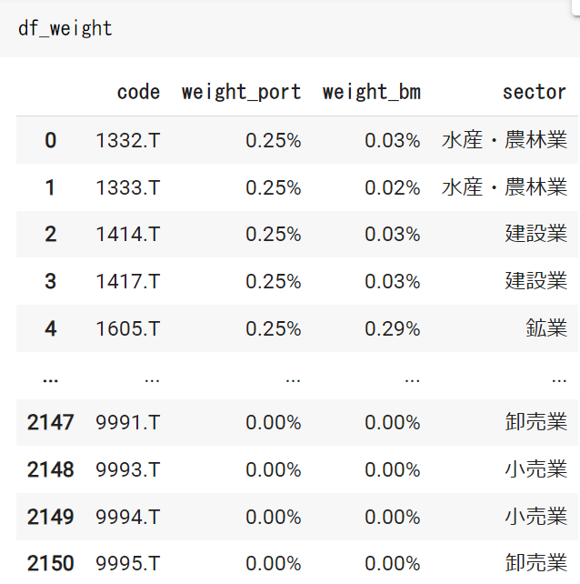
これらをまとめた情報であるdf_weightは次のようになります。
続いて、リターンデータをYahoo Financeから取得します。
from datetime import datetime, timedelta

today = datetime.now()
# 月初日を計算
first_day_of_month = today.replace(day=1)
date_s  =  first_day_of_month.strftime("%Y-%m-%d")
price = yf.download(list(df_weight['code']), start=date_s)
rtn = pd.DataFrame(price.iloc[-1,:]['Adj Close'] / price.iloc[0,:]['Adj Close'] - 1 ).reset_index()
rtn.columns = ['code','rtn']
データの準備が整いました。
ブリンソン型の要因分析
まずは取得したデータを整理し、ベンチマークリターンとポートフォリオリターンを作成します。
続いて、セクターごとのポートフォリオのリターンと、ベンチマークのリターンも計算しておきます。
df = pd.merge(df_weight, rtn, on=['code'])

def cal_weight(x, name='weight'):
    return  x[name]/x[name].sum()

weight_sector_bm = pd.DataFrame(df.set_index('code').groupby('sector').apply(cal_weight, name='weight_bm')).reset_index()
weight_sector_port = pd.DataFrame(df.set_index('code').groupby('sector').apply(cal_weight, name='weight_port')).reset_index()
df = pd.merge(df, weight_sector_bm.loc[:,['code','weight_bm']],on='code',suffixes=['','_sector'])
df = pd.merge(df, weight_sector_port.loc[:,['code','weight_port']],on='code',suffixes=['','_sector'])
df['rtn_bm'] = df['rtn'] * df['weight_bm_sector']
df['rtn_port'] = df['rtn'] * df['weight_port_sector']
df['weight_rtn_bm'] = df['weight_bm'] * df['rtn']
df['weight_rtn_port'] = df['weight_port'] * df['rtn']
df_sector = df[['weight_port','weight_bm','rtn_port', 'rtn_bm', 'sector','weight_rtn_bm','weight_rtn_port']].groupby('sector').sum()
アロケーション効果、セレクション効果、複合効果をそれぞれ計算します。
sector_effect = pd.DataFrame((df_sector['weight_port'] - df_sector['weight_bm']) * df_sector['rtn_bm'], columns=['アロケーション効果'])
selection_effect = pd.DataFrame((df_sector['rtn_port'] - df_sector['rtn_bm']) * df_sector['weight_bm'], columns=['銘柄選択効果'])
comb_effect =  pd.DataFrame((df_sector['weight_port'] - df_sector['weight_bm']) * (df_sector['rtn_port'] - df_sector['rtn_bm']), columns=['複合効果'])
ベンチマークのリターン、ポートフォリオのリターンをそれぞれ計算し、結果をまとめます。
bm_rtn = (df['weight_bm'] * df['rtn']).sum()
port_rtn = (df['weight_port'] * df['rtn']).sum()
print(f'benchmark return : {bm_rtn:.2%}')
print(f'portfolio return : {port_rtn:.2%}')
result = pd.merge(sector_effect, selection_effect,right_index=True, left_index=True)
result = pd.merge(result, comb_effect, right_index=True, left_index=True)
result = pd.merge(df_sector['weight_rtn_bm'], result, right_index=True, left_index=True)
result = pd.merge(df_sector['weight_rtn_port'], result, right_index=True, left_index=True)
result.columns = ['ポートフォリオ','ベンチマーク','アロケーション効果','銘柄選択効果','複合効果']

result.loc['合計',['ポートフォリオ','ベンチマーク','アロケーション効果','銘柄選択効果','複合効果']] = result.sum()
実行すると次のような結果を得られます。

今回のコードはこちらのGoogle Colabで確認できます。